The Graph Coloring Problem (GCP)

The graph coloring problem (GCP) refers to the problem of finding the coloring of an undirected, unweighted graph with the minimal number of colors (namely, the chromatic number). To solve the GCP problem, we implement the Greedy Coloring (GC) algorithm and the Recursive Largest First (RLF) algorithm. Moreover, we also formulate the GCP problem into an Integer Programming (IP) problem and attempt to solve it. Finally, the performances of the algorithms are compared in terms of optimality and computational time.

Heuristic algorithms

We will describe two heuristic algorithms for the GCP problem, namely the Greedy Coloring (GC) algorithm and the Recursive Largest First (RLF) algorithm. The GC iterates over vertices of the graph, and tries to use existing colors as much as possible provided that all neighbors have not occupied all. In contrast, the RLF iterates over colors, and in each iteration it tries to assign the color to as many vertices as possible.

Before walking into the algorithms we introduce the notations used throughout the paper. Consider a graph \(G = (V,E)\) with vertex set \(V = \{ v_1, \cdots, v_n \}\) and edge set \(E\). The color function \(\phi(\cdot)\) maps from a vertex to a color. For simplicity, and w.l.o.g., we set the color set to be the set of positive natural numbers \(\mathbb{N}_+\).

Greedy Coloring (GC)

The GC algorithm is stated in the following box.

function Greedy-Coloring (graph \(G = (V, E)\)):

     initialise set \(\phi(v_1) = 1\) and \(\phi(v_i)=0\) for all \(2 \leq i \leq n\)

     iterate \(2 \leq i \leq n\)

let \(\phi(v_i) = \min \{ k \in \mathbb{N}_+ \\| \phi(v_j) \neq k\) if \(v_i v_j \in E \}\);

return \(\phi(v)\)

Thus, the GC algorithm ends up with a \(k\)-coloring where

\begin{equation} k = \max_{v_i \in V} \phi (v_i). \end{equation}

Note that the GC algorithm aims for optimality by assigning the smallest possible color to a vertex in one iteration.

One important feature of the GC algorithm is that the pre-defined order of vertices completely decides the order of being colored. Different orders of being colored might result in different minimal numbers of colors. In other words, the optimality of the GC algorithm is not guaranteed, and is sensitive to the order of vertices to be colored.

Recursive Largest First (RLF)

Unlike GC that iterates over vertices, the RLF algorithm iterates over colors and maximises the number of vertices that can be assigned a color in each iteration. The algorithm details are shown in the following box.

function RLF (graph \(G = (V,E)\)):

     initialise calculate the degree for each vertex, select the vertex with the largest degree for coloring. The largest degree vertex is assigned the active_color = 1. Define init_vertex as the colored vertex;

     iterate until all vertices are colored

find all adjacent vertices of the init_vertex and add to a set \(A\);

find all vertices that are not adjacent to the init_vertex and add to a set \(U\);

     iterate until \(U\) is empty

calculate the number of adjacent vertices which are in \(A\) for each vertex in \(U\). After that, the uncolored vertex with maximum adjacent vertices (which are in \(A\)) in \(U\) is selected for coloring. The selected vertex is colored with the active_color;

remove the colored vertex and its adjacent vertices from \(U\), and add them to \(A\);

update active_color = active_color + 1;

calculate the number of adjacent vertices which are uncolored for every uncolored vertex. After that, the uncolored vertex having maximum uncolored adjacent vertices is selected for coloring process. If more than one vertex satisfies this condition, the vertex with the largest degree among them is selected. Color the selected vertex with active_color, and update init_vertex with the colored vertex;

return color assignment

The primary idea of the RLF algorithm is to assign one color to as many vertices as possible and then move to assigning the next color. More than that, in one color assignment, it defines the order of vertices to be colored basically according to vertex degree. Vertex with larger degree has higher priority of being colored. We expect that RLF shall be much less sensitive to the initial ordering of vertices than GC.

Integer programming formulation

We can formulate the GCP into an integer programming (IP) problem. Thereafter, solving the IP problem results in the chromatic number.

In a graph with vertex set \(V = \{ v_1, \cdots, v_n \}\), we need at most \(n\) colors to color all the vertices. We introduce binary variables \(y_k\) for \(k=1,\cdots,n\) such that

\[y_k = \begin{cases} 1, \text{ color } k \text{ is used}, \\ 0, \text{ color } k \text{ is not used}. \end{cases}\]

Furthermore, we introduce binary variables \(x_{ik}\) to indicate whether vertex \(i\) is assigned color \(k\), for \(i,k=1,\cdots,n\)

\[x_{ik} = \begin{cases} 1, \text{ vertex } i \text{ is assigned color } k, \\ 0, \text{ vertex } i \text{ is not assigned color } k. \end{cases}\]

The resulting IP is

\begin{align} \min_{x,y} \quad & \sum_{j=1}^n y_k \label{eq:IP_obj}
\end{align} \begin{align} \text{s.t.} \quad & \sum_{k=1}^n x_{ik} = 1, & \forall i = 1,\cdots,n; \label{eq:IP_1to1}
\end{align} \begin{align} & x_{ik} + x_{jk} \leq 1, & \forall v_i v_j \in E, k = 1,\cdots,n; \label{eq:IP_noNeighbor}
\end{align} \begin{align} & x_{ik} - y_k \leq 0, & \forall i,k = 1,\cdots,n; \label{eq:IP_relation}
\end{align} \begin{align} & 0 \leq x_{ik}, y_k \leq 1, & \forall i,k = 1,\cdots,n; \label{eq:IP_bin1}
\end{align} \begin{align} & x_{ik}, y_k \in \mathbb{Z}, & \forall i,k = 1,\cdots,n. \label{eq:IP_bin2} \end{align}

The objective \eqref{eq:IP_obj} is to minimise the number of colors to be used. Constraint \eqref{eq:IP_1to1} addresses that each vertex is assigned one and only one color. The next constraint \eqref{eq:IP_noNeighbor} then forbids neighbor vertices from being assigned the same color. There should then be a constraint concerning the relationship between \(x_{ik}\) and \(y_k\). Constraint \eqref{eq:IP_relation} does the job: if color \(k\) is not used, then no vertices shall receive the color \(k\). The last two constraints \eqref{eq:IP_bin1} and \eqref{eq:IP_bin2} corresponds to the binary property of variables \(x\) and \(y\).

The IP formulation of the GCP has \(\mathcal{O}(n^2) \sim \mathcal{O}(n^3)\) number of constraints, depending on the completeness of the graph. We can expect the solving complexity to increase dramatically as the graph size \(n\) grows.

Case study - Petersen graph

We apply the two heuristic graph algorithms GC and RLF, and the IP approach to the Petersen graph, as shown in Figure 1.

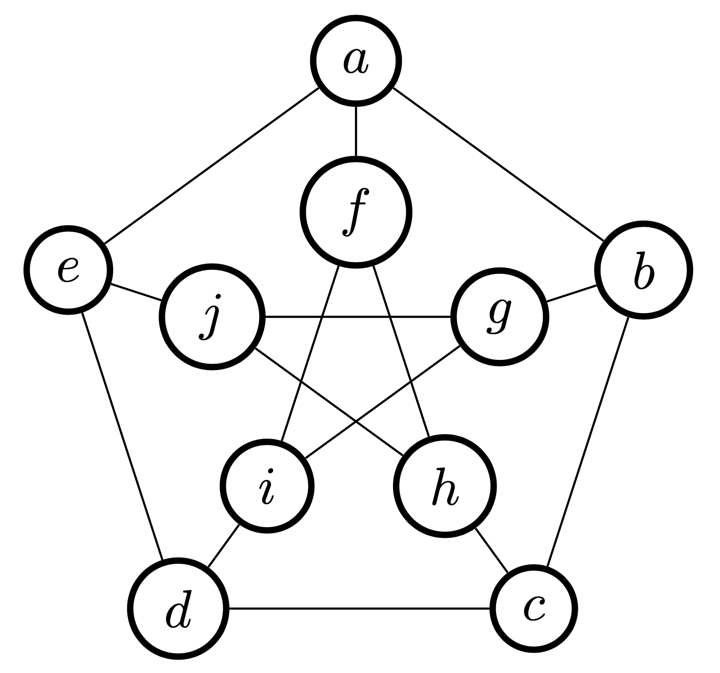
Figure 1 - Petersen graph.

We report the results from the three algorithms in \Cref{tab:PerformPetersen}. All three algorithms agree on the minimal number of colors, namely 3. In terms of computational speed, IP is the slowest. GC is slightly faster than RLF.

Algorithm	\(k\)-coloring	Time (seconds)
GC	3	0.0002
RLF	3	0.0005
IP	3	0.1476

Table 1 - Algorithm performance on the Petersen graph.

The LP relaxation problem of the IP can be obtained by removing the integral constraint (\ref{eq:IP_bin2}). Solving the LP relaxation problem, we get a result:

\[\begin{equation} y_{k} = \begin{cases} 0.5, &\quad k =1,2,\\ 0, &\quad k = 3,\cdots,n, \end{cases} \label{eq:LP_y} \end{equation}\] \[\begin{align} x_{ik} & = \begin{cases} 0.5, &\quad k=1,2, \text{ }\forall i, \\ 0, &\quad k = 3,\cdots,n, \text{ }\forall i, \end{cases} \label{eq:LP_x} \end{align}\]

where \(n=10\) for the Petersen graph. Thus, the optimal objective value of the LP relaxation problem is 1, which is quite different from the optimum of the IP. In fact, this optimal solution is the optimal solution for LP relaxation problems of any graph. If forgetting the graph scale \(n\) for a moment, the only constraint concerning the topology of a graph is (\ref{eq:IP_noNeighbor}) that specifies no neighbor vertices shall receive the same color. Regardless of how edges are configured in \(E\), the optimal solution (\ref{eq:LP_x}) is always feasible under constraint (\ref{eq:IP_noNeighbor}). We can argue for the optimality of the solution by proof of contradiction.

Case study - Erdos-Renyi graph

To study the scaling of the three algorithms to the GCP, we implement them to the Erdos-Renyi graph \(G(n,p)\) for varying \(n\) and fixed probability \(p=0.7\).

Since the Erdos-Renyi graph is a random graph, we run each algorithm for 100 realisations and compare among algorithms by average performance and its standard deviation. The performance to be compared includes the minimal number of colors and computational time.

Firstly, we compare the two heuristic algorithms. The average minimal number of colors achieved is shown in Figure 2. \(x\)-axis indicates the scale of graph \(n\), and \(y\)-axis marks the number of colors. The solid line represents the average minimal number of colors achieved. Furthermore, the error bar is also attached on the solid line, implying the range of two standard deviations (where 95% of data will fall within assuming that data follow normal distribution).

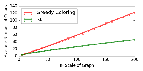
Figure 2 - Minimal number of colors achieved.

Apparently RLF performs better and better than the greedy algorithm in finding the minimal number of colors as graph is getting larger and larger. In particular, in a \(G(200, 0.7)\) graph, GC says it requires on average 123.28 colors to color the graph, while RLF says 46.03 is enough. The standard deviations of results from both algorithms are relatively small, indicating that both algorithms are stable.

Figure 3 then shows the average computational time comparison between the two algorithms. The computational time of both GC and RLF increases nonlinearly with \(n\). It is observed that RLF becomes faster then GC when the graph has more then 100 vertices. Indeed, though it is not quite observable in Figure 3, that GC is slightly faster than RLF when the graph has no more than 90 vertices. The performance table for the Petersen graph (Table 1) agrees with this observation, where GC elapsed in 0.0002 seconds while RLF elapsed in 0.0005 seconds. Anyway, the slight outperformance of GC applied in small-scaled graph seems negligible. The standard deviations of results from both algorithms are relatively small, indicating that both algorithms are stable.

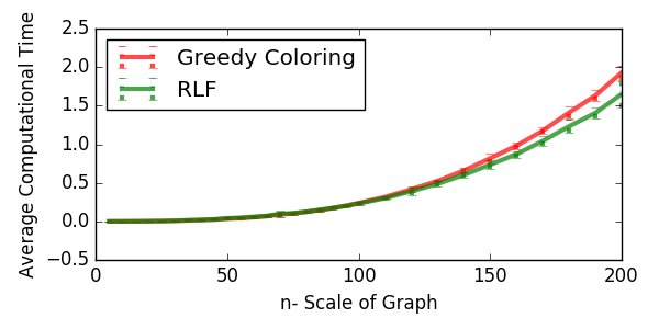
Figure 3 - Computational time.

Note that, all curves in Figure 2 and Figure 3 look relatively smooth and trendy. This shows that 100 realisations are a proper and sufficient choice to assess the algorithms performance for random graphs.

We add the performance of IP to comparison. However, in this comparison, we are unable to increase the graph size to 200 as we did for the heuristic algorithms. The reason is that the computational time of IP increases dramatically as graph gets larger. In our numerical experiments, we use 100 different random generator seeds to control realisations. The IP can produce results within reasonably stable and short time period (\(\leq 5\) secs) for each realisation at small \(n\). However, when increasing \(n\) to 15, it takes around 20 mins to get results for some realisation but takes only seconds for others. This implies that the speed and stability of the IP becomes very sensitive to graph topology as graph sizes grow.

In Figure 4, we show the average minimal number of colors achieved by each approach. Due to the instability of IP we observed when \(n \geq 15\), we only run 10 realisations (which exclude those requiring unaffordably long elapsed time) for graphs with more than 14 vertices. This causes the non-smooth behaviours of all curves for \(n \geq 15\).

Since IP will always give the chromatic number, we use IP as the benchmark to show how far away each heuristic algorithm is from the optimality. From Figure 4, we see that RLF agrees with IP when \(n \leq 22\), and starts to produce less optimal result when graph size grows larger. GC’s result starts to diverge from IP’s results significantly since \(n \geq 9\).

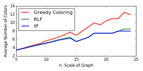
Figure 4 - Minimal number of colors achieved.

Looking at the average computational time, as shown in Figure 5, IP becomes much more expensive than the other two heuristic algorithms. What’s worse, as addressed before, IP requires 20 mins for solving some realisation of \(G(15,0.7)\). Figure 5 turns out only to show some “fast” realisations.

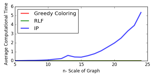
Figure 5 - Computational time.

Conclusion

We have implemented the Greedy Coloring (GC) algorithm, the Recursive Largest First (RLF) algorithm, and Integer Programming (IP) to solve the graph coloring problem. In particular, we compare these 3 algorithms by the minimal number of colors achieved as well as computational time. The GC and RLF algorithms are heuristic and do not guarantee the minimal number of colors achieved is the chromatic number. RLF beats GC more and more when the graph size scales up, in terms of both optimality and speed. Integer programming always gives the chromatic number, as long as the formulated IP can be solved at optimality. However, the computational time of the IP approach can be unaffordable as the graph size scales up.