Hanging catenary
A catenary is the curve that an idealised hanging chain or cable assumes under its own weight when supported only at its ends. For example, a stressed ribbon bridge hanging between pillars on either side of a river forms a shape of catenary. The catenary shape can be derived by minimising the total energy of the hanging chain. We would like to formulate a discrete energy objective and minimise it numerically.
Modelling the shape
We model a catenary of \(n+1\) beams in a 2-dimensional \((x,y)\) plane, with the first beam fixed at the origin and the final beam fixed at a fraction \(\gamma \in (0,1)\) of the total length of all the beams. Suppose each beam is of length \(L\) and of mass \(m\). Let \((x_i, y_i)\), \(i=1,\cdots,n+1\) be the coordinates of the end of the beams and \((x_0,y_0) = (0,0)\) the coordinate of the start point of the first beam. Assuming that the gravity acts at the middle of each beam, then we have the gravitational potential energy
\begin{equation} E_\text{G} = \sum_{i=1}^{n} mg \cdot \frac{1}{2}(y_{i-1} + y_{i}), \end{equation}
where \(g\) is the gravitational constant. Hence, the resulting problem minimises the energy of the system \(E_\text{G}\). Since \(mg\) is constant, we define the problem as
\begin{equation} \min_{x,y} \quad \frac{1}{2} y_0 + y_1 + \cdots + y_n + \frac{1}{2} y_{n+1} \label{eq:MinProblem} \end{equation}
\[\text{subject to} \quad (x_0, y_0) = (0,0),\] \[(x_{n+1}, y_{n+1}) = (\gamma (n+1)L, Y),\] \[(x_i - x_{i+1})^2 + (y_i - y_{i+1})^2 = L^2, \forall i = 0,\cdots, n.\]Here \(Y\) is a constant indicating the vertical position of the end of the final beam.
Numerical optimisation
We solve the constrained minimisation problem (\ref{eq:MinProblem}) numerically given values of parameters \(n\), \(\gamma\), \(L\), \(Y\). To be specific, we use MATLAB Optimization Toolbox to implement the interior-point algorithm. It is of our interest to study the optimisation performance under different configurations.
We define the optimisation configuration matrix in Table 1.
| Parameter | Description | Default |
|---|---|---|
| \(T_\text{1st}\) | Termination tolerance on the first-order optimality | 1e-6 |
| \(T_\text{C}\) | Termination tolerance on the constraint violation | 1e-6 |
| \((\mathbf{x}^0, \mathbf{y}^0)\) | Starting points | (0,0) |
| \(S_\text{G}\) | Supplying analytical gradients | false |
| \(S_\text{GH}\) | Supplying analytical gradients and Hessian | false |
Table 1 - Optimisation configuration matrix.
While the default values are given in the last column, we are about to investigate how the optimisation performs by adjusting these parameters. Note that we assume very small tolerant step size and very large tolerant number of iterations and function evaluations, so that the numerical process will only terminate by satisfying the pre-defined tolerances (i.e. \(T_\text{1st}\) and \(T_\text{C}\)). In fact, we take the number of iterations and function evaluations as our key measures of the algorithm efficiency.
Table 2 lists the interested measures of optimisation performance. Given fixed stopping criteria, a more efficient process will terminate with less iterations (\(N_\text{I}\)) and function evaluations (\(N_\text{F}\)), while a more effective process will end up will smaller first-order derivative (\(E_\text{1st}\)) and constraint violations (\(E_\text{C}\)).
| Parameter | Description |
|---|---|
| \(N_\text{I}\) | Number of iterations |
| \(N_\text{F}\) | Number of function evaluations |
| \(E_\text{1st}\) | Measure of the realised first-order optimality |
| \(E_\text{C}\) | Maximum of constraint function violations |
Table 2 - Optimisation performance matrix.
To proceed with the numerical process, we assign instance values to the model parameters as listed in Table 3. We will modify some default values to study corresponding impact on the optimisation performance.
| Parameter | \(n\) | \(\gamma\) | \(L\) | \(Y\) |
| Value | 19 | 0.8 | 1 | 5 |
Table 3 - Default values of the model parameters.
Optimisation with default configurations
We start from looking at the results with default configs. Figure 1 displays the resulted shape, and Figure 2 traces the evolution of function values and first-order optimality over iterations.
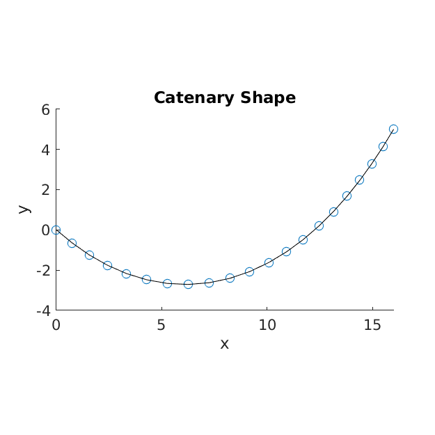
Figure 1 - Catenary shape.
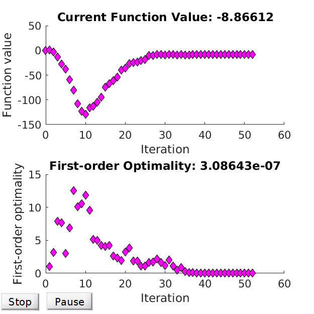
Figure 2 - Optimisation performance.
Supplying gradients and Hessian
The default configs do not admit gradients or Hessian, in which case the solvers estimate them via finite differences. The estimation is time-consuming and can be less accurate for higher order of derivatives. In the catenary problem, it is possible to derive analytical form of gradients and Hessian for both objectives and constraints. We monitor changes in optimisation performance by including gradients (\(S_\text{G} = \text{true}\)) and Hessian (\(S_\text{GH} = \text{true}\)) in sequence.
| \(n=19\) | \(n=49\) | |||
|---|---|---|---|---|
| Solver | \(N_\text{I}\) | \(N_\text{F}\) | \(N_\text{I}\) | \(N_\text{F}\) |
| Default | 51 | 2299 | 565 | 61639 |
| \(S_\text{G} = \text{true}\) | 65 | 213 | 152 | 528 |
| \(S_\text{GH} = \text{true}\) | 41 | 88 | 106 | 174 |
Table 4 - Performance with gradients and Hessian
Table 4 shows the number of iterations and function evaluations by different solvers, given different values of \(n\). In both cases, the number of iterations is reduced dramatically after including analytical Hessian, but increases a bit if only including gradients. Nevertheless, including gradients avoids a substantial amount of function evaluations. Moreover, when \(n\) is larger, the efficiency introduced by adding gradients and Hessian becomes more noticeable.
Meanwhile, we observe that, for default solver, \(N_\text{I}\) and \(N_\text{F}\) increases much faster when \(n\) grows. We expect that the computational complexity will soon become unaffordable if \(n\) becomes \(500, 1000\) or more. We attempt to reduce computing complexity by adapting the initial points.
Modifying initial points
Instead of giving trivial initial guess, we make a wiser choice for at least \(\mathbf{x}^0\). A physically meaningful choice would be that \(x_i\)’s are evenly distributed within the interval \([x_0, x_{n+1}]\). Following this choice, we modify Table 4 to Table 5.
| \(n=19\) | \(n=49\) | |||
|---|---|---|---|---|
| Solver | \(N_\text{I}\) | \(N_\text{F}\) | \(N_\text{I}\) | \(N_\text{F}\) |
| Default | 52 | 2331 | 140 | 14782 |
| \(S_\text{G} = \text{true}\) | 52 | 120 | 152 | 559 |
| \(S_\text{GH} = \text{true}\) | 10 | 16 | 13 | 18 |
Table 5 - Performance with wise initial points
The changes due to initial points are significant, especially in the case of larger \(n\). In particular, the solver with gradients and Hessian gets most improvement.
So far the observed most efficient numerical scheme is the gradient and Hessian solver with evenly distributed initial points \(\mathbf{x}^0\). We will further test the robustness of this scheme by scaling up the catenary problem, i.e. to allow \(n\) to grow to a very large number.
Increasing the number of beams
Let \(Y=0\) rather then 5 such that the initial guess probably makes more sense. We run the chosen solver for \(n=99,\cdots,9999\) and show the number of iterations and function evaluations in Table 6. The chosen numerical scheme proves to be super efficient since the number of iterations seems follow a logarithmic growth with \(n\).
| \(n\) | 9 | 49 | 99 | 499 | 999 | 4999 | 9999 |
| \(N_\text{I}\) | 8 | 11 | 12 | 14 | 15 | 18 | 19 |
| \(N_\text{F}\) | 13 | 16 | 17 | 19 | 20 | 23 | 24 |
Table 6 - Performance under different \(n\).
Experiment on model parameter Y
Suppose we set \(Y\) back to the default value 5 and re-run the same numerical scheme, will we get the same performance? The answer is no. In fact, \(n=99\) leads to \(N_\text{I} = 33\), \(n=499\) leads to \(N_\text{I} = 501\), and \(n=999\) leads to \(N_\text{I} = 1445\). This evidence implies the key role that the initial points play in the scheme. Our initial guess might not fit the case where \(Y=5\) well because more beams tend to group near the right side, far more from the assumption of even distribution. It is expected that our numerical scheme is less efficient given larger \(\\|Y\\|\) (either larger positive \(Y\) or smaller negative \(Y\)).
Experiment on model parameter gamma
Will the numerical optimisation performance be invariant with the model parameter \(\gamma\)? The answer is no, as well. Similar to \(Y\), the value of \(\gamma\) has a saying on the quality of our initial guess. The smaller the \(\gamma\) is, in physical sense more beams will stay closer to the two sides, so that the initial guess of even horizontal distribution is more unrealistic. This is evidenced by the observations shown in Table 7, where we run the numerical scheme given different \(\gamma\) (we fix \(n=499\)).
| \(\gamma\) | 0.01 | 0.1 | 0.2 | 0.5 | 0.7 | 0.8 | 0.9 | 0.99 |
| \(N_\text{I}\) | \(>3000\) | 270 | 242 | 26 | 14 | 14 | 15 | 17 |
| \(N_\text{F}\) | \(>5000\) | 807 | 578 | 55 | 19 | 19 | 20 | 22 |
Table 7 - Performance under different \(\gamma\)
Termination tolerance and realised error
Finally we look at the comparison between termination tolerance (\(T_\text{1st}\) and \(T_\text{C}\)) and realised error (\(E_\text{1st}\) and \(E_\text{C}\)). We study the case where \(n=499\), \(Y=0\) and all the other parameters reserve default values.
Recall that we assume very small tolerant step size and very large tolerant number of iterations and function evaluations. In implementation, we input 1e-100 for the stepsize, and 1e10 for the number of iterations and function evaluations. Now we lift \(T_\text{1st}\) and \(T_\text{C}\) up to 1e-100, and obtain results shown in Figure 3. The optimisation stopped because the relative changes in all elements of \(\mathbf{x}\) are less than \texttt{1e-100}. Hence, it seems there’s a limit on achievable levels for \(E_\text{1st}\) and \(E_\text{C}\). Meanwhile, Figure 3 provides a good guidance to know how many iterations are required for the desired tolerance \(T_\text{1st}\) and \(T_\text{C}\).
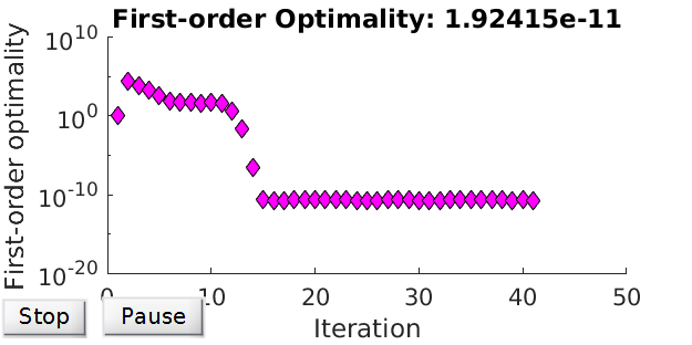
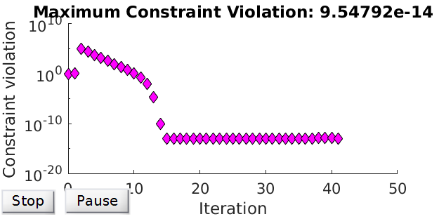
Figure 3 - Realised errors over iterations.
Conclusion
We propose a numerical minimisation scheme to solve the catenary problem. We observe that including gradients and Hessian can largely improve the efficiency of the scheme, and such improvement is more significant in large-scaled problem. Moreover, initial guess also plays a key role in improving efficiency, though it is difficult to come up with a perfect one.