Ribbon bridge
A ribbon bridge hangs between pillars on either side of a river. We would like to model the shape of the bridge by deriving a governing differential equation from the energy minimisation approach. Thereafter we solve the differential equation and arrive at a formula for the shape.
Modelling the shape
We model the shape of a ribbon bridge in a 2-dimensional \((x,y)\) plane. Denote the height of the bridge at horizontal position \(x\) as \(y(x)\), and the bridge spans from \(x_a\) to \(x_b\). Therefore, we have the gravitational potential energy \begin{equation} E_\text{G} = \int_{x_a}^{x_b} \rho g y \sqrt{1 + (y’)^2} \mathrm{d} x, \label{eq:GravPotentialEnergy} \end{equation} where \(\rho\) is the mass density (mass per unit length) of the bridge and \(g\) is the gravitational constant. By using the fact that the length of the bridge is a fixed constant \(L\), we formulate \begin{equation} \int_{x_a}^{x_b} \sqrt{1 + (y’)^2} \mathrm{d} x = L. \label{eq:ConstantLength} \end{equation}
The idea is then to find a formulation for \(y\) such that the energy of the system, \(E_\text{G}\) in (\ref{eq:GravPotentialEnergy}), is minimised with the constraint specified as (\ref{eq:ConstantLength}). This is equivalent to \begin{equation} \min_{y} \int_{x_a}^{x_b} f(y,y’) - \frac{\lambda L}{x_b - x_a} \mathrm{d} x, \label{eq:MinimisationProblem} \end{equation} where \(\lambda\) is the Lagrangian multiplier, and \begin{equation} f(y, y’) = ( \rho g y + \lambda ) \sqrt{1 + (y’)^2}. \end{equation}
The Beltrami Identity states that the minimal is reached when (\ref{eq:BeltramiIdentity}) holds for some constant \(c\), \begin{equation} f - y’ \frac{\partial f}{\partial y’} = c, \label{eq:BeltramiIdentity} \end{equation} which leads to \begin{equation} \rho g y + \lambda = c \sqrt{1 + (y’)^2}. \label{eq:GoverningODE} \end{equation}
We take square on both sides of the equation (\ref{eq:GoverningODE}) and then take first derivative against \(x\) on both sides, to obtain \begin{equation} y’’ - \left( \frac{\rho g}{c} \right)^2 y = \frac{\rho g \lambda}{c^2}. \label{eq:GoverningODE1} \end{equation} Note that we omit the physically-unrealistic solution \(y'=0\) in the derivation to (\ref{eq:GoverningODE1}). The complete solution \(y\) consists of a complementary solution \(y_c\) and a particular solution \(y_p\), namely \(y = y_c + y_p\). \(y_c\) is the solution to the corresponding homogeneous problem and have the form \begin{equation} y_c = A \cosh \left( \frac{\rho g}{c} (x-x_0) \right), \end{equation} where the constants \(A\) and \(x_0\) remain to be determined. Substituting \(y_c\) into (\ref{eq:GoverningODE}) yields \(A = c / \rho g\). The particular solution shall have a form \(y_p = B\) for a constant \(B\). Plugging \(y_p\) into (\ref{eq:GoverningODE1}) gives \(B = - \lambda / \rho g\). Hence, \begin{equation} y = \frac{c}{\rho g} \cosh \left( \frac{\rho g}{c} (x - x_0) \right) - \frac{\lambda}{\rho g} \label{eq:ShapeSolution} \end{equation} is the solution to the bridge shape governing equation (\ref{eq:GoverningODE}) with three constants \(c\), \(x_0\) and \(\lambda\) to be determined by boundary conditions.
Shape calibration
We calibrate the shape solution (\ref{eq:ShapeSolution}) to a real world stress ribbon bridge by choosing parameters \(c\), \(x_0\) and \(\lambda\).
We look at the lignon-Loex Bridge, that crosses the river Rhone, and is situated in the suburbs of Geneva. It is formed by a stress ribbon of one span of length \(S=136\text{m}\); the sag at mid-span is \(D=5.6\text{m}\). We assume the two ends of the bridge are at the same horizon, and put the bridge in the (\(x\),\(y\)) coordinate such that \(x_a = 0\) and \(x_b = S\). Therefore, we impose three boundary conditions to (\ref{eq:ShapeSolution}), \begin{equation} y(x_a) = 0, \quad y(x_b) = 0, \quad y(\frac{S}{2}) = -D. \label{eq:Boundary} \end{equation} Denoting \(c^* = c/ \rho g\), \(\lambda^* = \lambda / \rho g\), we plug the boundary conditions \ref{eq:Boundary} into \ref{eq:ShapeSolution} and get numerical results. \begin{equation} c* \approx 413.79 \mathrm{m}^{-1}, \quad x_0 \approx 68 \mathrm{m}, \quad \lambda^* \approx 419.39 \mathrm{m}^{-1}. \end{equation}
The gravitational constant \(g\) is approximately \(9.8 \text{m}/\text{s}^2\), and the density of the bridge (made of concrete) is around \(2400 \mathrm{kg}/\mathrm{m}^3\). Assuming the bridge has an average width of \(2\)m and thickness of \(0.5\)m, then the density per unit length is \(\rho = 2400 \mathrm{kg}/\mathrm{m}\). Therefore, \begin{equation} c \approx 973227 \mathrm{N}, \quad \lambda \approx 986399 \mathrm{N}. \end{equation}
Moreover, we show the plot of the calibrated shape in Figure 1.
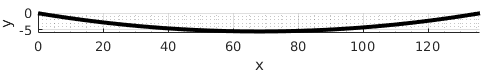
Figure 1 - Calibrated shape.
\(x_0\) is the midpoint of \(x_a\) and \(x_b\), the two endpoints of the bridge. The value of \(c\) seems differ little from the value of \(\lambda\). In fact, by initialising the coordinate properly, we can make \(c = \lambda\). For example, let \begin{equation} y(x_a=-\frac{S}{2} + x_0) = D, \quad y(x_b=\frac{S}{2} + x_0) = D, \quad y(x_0) = 0, \end{equation} we can show \(c = \lambda\).
The unit of \(c\) and \(\lambda\) is Newton, by matching the dimension in the governing differential equation. Indeed, the Lagrangian multiplier \(\lambda\) represents a meaningful physical quantity in this scenario. We illustrate in the next section.
Interpreting lambda
We know from dimensional analysis that \(\lambda\) represents a force. The next question is, what force exactly?
To demonstrate this, we consider the bridge shape in a slightly different situation. Now the bridge is pinned at one end, but at the other end the bridge is free to slide along the top of the pillar (i.e. the total bridge length between the pillars can change). We apply a constant horizontal force \(T\) to this end of the bridge. In this situation, the total energy of the system is composed of the gravitational potential energy (\ref{eq:GravPotentialEnergy}) and the work done by the horizontal force \(T\), which is
\begin{equation} W = T \cdot \Delta L = T(L - \int_{x_a}^{x_b} \sqrt{1+(y’)^2} \mathrm{d}x). \end{equation} and therefore the total energy is \begin{equation} E_\text{Tot} = E_\text{G} - W. \end{equation} Hence, we are seeking for \(y(x)\) that minimises the total energy \(E_\text{Tot}\), namely, \begin{equation} \min_{y} \int_{x_a}^{x_b} (\rho g y + T) \sqrt{1+(y’)^2} - \frac{TL}{x_b - x_a} \mathrm{d} x. \label{eq:Minimisation2} \end{equation}
Comparing (\ref{eq:Minimisation2}) with the minimisation problem (\ref{eq:MinimisationProblem}) defined in the previous scenario, they become identical if we let \begin{equation} \lambda = T. \end{equation}
Hence, it is reasonably to interpret the Lagrangian multiplier \(\lambda\) as the tension force transmitted through the bridge.
Conclusion
We derive the shape of a hanging ribbon bridge by minimising the total energy of the bridge system subject to constraints. To solve the constrained minimisation problem, we have used Lagrangian multiplier, which can be interpreted as tension force transmitted through the bridge. We also calibrate the shape solution to a real-world stress ribbon bridge, and estimate a typical magnitude for the tension force.