Solving a linear system
To solve a linear system \(Ax=b\), we can either invert the coefficient matrix \(A\) and multiply \(b\), or numerically approximate the roots by iterative methods. In the first approach, matrix inversion is always a pain, which we possibly mitigate by matrix factorizations on \(A\). The concern of the second approach is the convergence of the numerical scheme, which depends on the properties of \(A\).
In this post, we study multiple algorithms for QR factorizations, SVD decomposition and iterative root solving. We implement the algorithms in MATLAB and compare their performance, along with the MATLAB performance of in-built functions.
QR factorization
An \(m \times n\) matrix \(A\) can be factorized as \begin{equation} A = QR, \end{equation} with \(Q\) unitary (such that \(Q^*Q = QQ^* = I\)) and \(R\) upper triangular. Given \(Q\) and \(R\), we solve \(Ax=b\) by multiplying by \(Q^*\) and back-solving \(Rx = Q^*b\).
We implement three algorithms and contrast their performances. Table 1 lists the three QR algorithms we study and the MATLAB in-built qr() function that returns \(Q\) and \(R\) given an \(A\). It is computationally much easier of inverting \(R\) than directly inverting \(A\).
| Algorithm | flops |
|---|---|
| Modified Gram-Schmidt | \(2mn^2\) |
| Householder reflections | \(2mn^2 - \frac{2}{3} n^3\) |
| Givens rotations | \(3mn^2 - n^3\) |
MATLAB qr() | \(3mn^2 - n^3\) |
Table 1 - List of QR algorithms.
We simulate a matrix \(A\) with exponentially-decayed singular values in the following ways:
- Simulate an \(m \times m\) matrix \(U\) and \(n \times n\) matrix \(V\) from independent standard Gaussian distribution.
- Define \(r = \min(m,n)\), construct an \(r \times r\) diagonal matrix \(D\) where \(D_{11} = 1/c\) and \(D_{(i+1)(i+1)} = D_{ii}/c\) for all \(2 \leq i \leq r\).
- Compute \(A = U(:,1:r) D V(:,1:r)^\top\).
By construction, the ordered diagonal element of the decomposed upper triangular matrix \(R\) should decay exponentially. Figure 1 displays the ordered diagonal elements of \(R\) computed from the four algorithms. In this instance, \(m=n=80\) and \(c=2\). Their values shown in \(y\)-axis is on log-scale for clearer illustration. We do observe the four algorithms highly agree with each other up to the 58th largest value. Afterwards, there are slight discrepancies, but at trivial level \(\exp(-40)\). Those differences shall be owe to machine error. Overall, the ordered diagonal elements of \(R\) do decay exponentially, as expected.
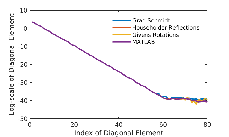
Figure 1 - Diagonal elements of \(R\) by various algorithms.
Iterative methods
To avoid matrix inversion, iterative methods are used to solve linear system numerically within specific tolerant errors. Table 2 lists the iterative methods we will cover in the followings. A brief description of the iteration form is shown in the table.
| Algorithm | Iterative Form |
|---|---|
| Jacobi | \(x^{(k+1)} = T_J x^{(k)} + c_J\) |
| Orthomin(1) | \(x^{(k+1)} = x^{(k)} + \alpha_k r^{(k)}\), \(r^{(k)} = b - A x^{(k)}\), \(\min || r^{(k+1)} ||_2\) along \(A r^{(k)}\) |
| Steepest Descent | \(x^{(k+1)} = x^{(k)} + \alpha_k r^{(k)}\), \(r^{(k)} = b - A x^{(k)}\), \(\min|| x - x^{(k+1)} ||_A\) along \(r^{(k)}\) |
| Orthomin(j) | \(x^{(k+1)} = x^{(k)} + \alpha_k p^{(k)}\), \(p^{(k)} = r^{(k)} - \sum_{q=k+1-j}^{k-1} \beta_q p^{(q)}\), \(r^{(k)} = b - A x^{(k)}\), \(\min || r^{(k+1)} ||_2\), \(A p^{(k)} \perp A p^{(q)}\), \(k+1-j \leq q < k\) |
| Conjugate Gradient | \(x^{(k+1)} = x^{(k)} + \alpha_k p^{(k)}\), \(p^{(k)} = r^{(k)} - \beta_{k-1} p^{(k-1)}\), \(r^{(k)} = b - A x^{(k)}\), \(\min || x- x^{(k+1)} ||_A\), \(r^{(k)} \perp r^{(q)}\), \(p^{(k)} \perp A p^{(q)}\), \(q < k\) |
| GMRES | \(x^{(k)} = Q_k y^{(k)}\), \(y^{(k)} = \text{arg}\min_y ||b-AQ_ky||\), \(\min || r^{(k)} ||_2\) over \(b+\mathcal{K}_k(b,A)\) |
Table 2 - List of Iterative Methods
Jacobi \(T\)
The Jacobi algorithm defines a matrix \(T_J\) and a vector \(c_J\), \begin{equation} T_J = I - D^{-1} A, \quad c_J = D^{-1} b, \end{equation} such that \(x=T_Jx+c_J\) is equivalent to \(Ax = b\). Note here \(D\) is the diagonal matrix of \(A\). Defining error as \(e^{(n)} = x - x(n)\) gives the formula \(e^{(n)} = T^n e^{(0)}\). Therefore, the convergence of the Jacobi algorithm hinges on understanding the properties of \(T\) so that \(\|T^n e^{(0)}\|\) converges to zero.
A theorem states that \(\|T^n\|\) converges to zero if and only if the spectral radius \(\rho(T) < 1\). In fact, this theorem is built on top of the fact that \begin{equation} \lim_{n \rightarrow \infty} ||T^n||^{\frac{1}{n}} = \rho(T), \label{eq:TConverge} \end{equation} in which case \(\|T^n\| = \rho^n(T) \rightarrow \infty\) as \(n \rightarrow \infty\) if \(\rho(T)<1\). To numerically demonstrate the property of \(T\) in \eqref{eq:TConverge}, we simulate a \(100\times 100\) matrix \(T\) from independent standard Gaussian distribution, and then calculate the ratio \(\|T^n\|^{1/n} / \rho(T)\) for different \(n\). Moreover, we try matrix norm defined in \(l^1\), \(l^2\) and \(l^{\infty}\).
In Figure 2, we plot the ratio defined under \(l^1\), \(l^2\) and \(l^\infty\)-norm for \(n = 2^j\) where \(j=1,2,\cdots8\). As \(n\) increases, all ratios decay to 1 almost around the same value of \(n\), though starting from different points. \(l^1\) and \(l^{\infty}\)-norm result in almost the same ratio along \(n\). This is expected from the definition of various matrix norms.
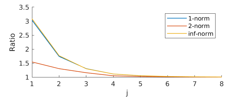
Figure 2 - Convergence of \(\|T^n\|^{1/n}\) to \(\rho(T)\).
Convergence performance of Jacobi, Orthomin(1) and Steepest Descent
Next we compare the rate of convergence of algorithm Jacobi, Orthomin(1) and Steepest Descent. The residual \(\|r^{(k)}\|\) at \(k\)-th iteration is defined as \(\|b-Ax^{(k)}\|\). In particular, we construct a \(1000\times 1000\) strictly row diagonal dominant (SRDD) matrix \(A\), and solve \(Ax=b\) (for some \(b\)) iteratively. The termination criteria is either the residual hits the tolerant error tol = 1e-8 or the the number of iterations hits the maximum max_iter = 1e6. Figure 3 shows how residual reduces over iteration. Note that all algorithms converge linear in log scale. Both Jacobi and Orthomin(1) converge at 6-th iteration, while Steepest Descent converges 1 iteration further. We further show how convergence over computational time in Figure 4. It seems to imply that the Steepest Descent algorithm not only takes more iterations, but also more time. It is not true in general.
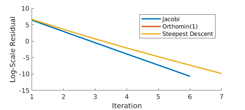
Figure 3 - Log-scale residual over iterations.
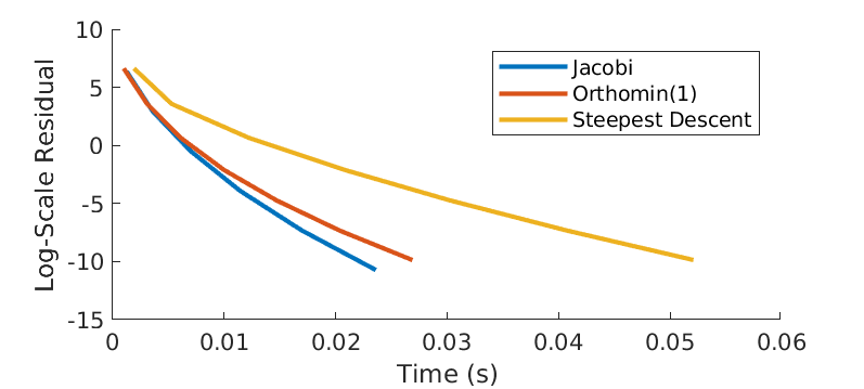
Figure 4 - Log-scale residual over time.
Recall the convergence theorem for the Jacobi algorithm, which says that if \(A\) is SRDD, then the algorithm converges to the solution of the linear system of equations \(A^{-1}b\) at a linear rate \(\|x^{(k)}-A^{-1}b\| \leq \mathcal{O}(\gamma^{k})\) with \(\gamma \leq \rho(T_J) < 1\). This is consistent with the observations in Figure 4.
Finally, we scale the problem by adjusting size of matrix \(A\) and see how the convergence time behaves for all the three algorithms along with the MATLAB in-built \(LU\) factorization function. Figure 5 displays the time of convergence with \(m\), the size of matrix. There is no surprise that the required time of convergence increases with matrix size, for all algorithms. However, the MATLAB in-built function is more sensitive to change in matrix size. In particular, when \(m\) exceeds around 120, the MATLAB function requires more and more time than the other 3 algorithms do for convergence. In addition, Jacobi gives worse convergence time than the other 2 as \(m\) scales up.
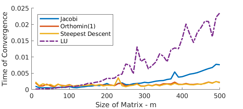
Figure 5 - Time of convergence.
Convergence performance of Orthomin(j) and Conjugate Gradient
The Orthomin(j) and the Conjugate Gradient algorithm can be viewed as an augmented version for Orthomin(1) and Steepest Descent, respectively, by optimizing the search direction to accelerate convergence.
First we take a close look at how \(j\) affects the convergence performance of the Orthomin(j) algorithm. We generate a symmetric \(1000 \times 1000\) matrix \(A\). Its diagonal forms a linear span from 1 to 2, and all the off-diagonal entries follow the independent standard Gaussian distribution. The termination criteria of iterative solving \(Ax=b\) is either the residual hits the tolerant error tol = 1e-8 or the the number of iterations hits the maximum max_iter = 1e6.
Figure 6 shows, at convergence, the number of iterations and computational time required for different \(j\). It shows strong evidence that the convergence rate (either measured in number of iterations or time) for Orthomin(j) is indifferent for any \(j \geq 2\). Nevertheless, Orthomim(1) performs significantly worse due to the lack of optimal search direction. Therefore, in the following analysis, we will primarily use Orthomin(2) algorithm in the comparison with other algorithms, without worrying too much about larger \(j\).
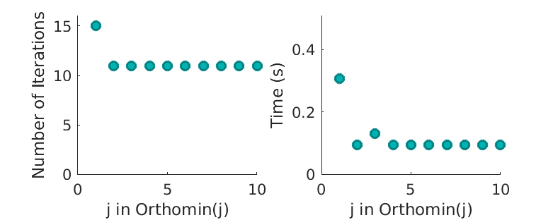
Figure 6 - Different \(j\) - convergence of Orthomin(j).
We contrast the Conjugate Gradient algorithm with Orthomin(2) and Orthomin(8) in in terms of convergence rate, as shown in Figure 7. As illustrated before, there shall be no difference between Orthomin(2) and Orthomin(8). In addition, we observe that the Conjugate Gradient algorithm has almost the same convergence as the other 2.
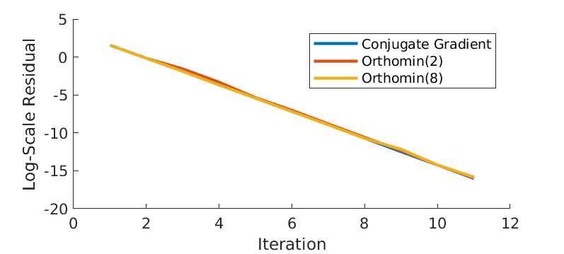
Figure 7 - Log-scale residual over iterations.
Finally, we scale the matrix size and see how convergence time changes for all algorithms. In addition, we also include MATLAB in-built \(LU\) factorization function into comparison. Figure 8 plots the time of convergence with \(m\), the size of matrix. There is no surprise that the required time of convergence increases with matrix size, for all algorithms. However, the MATLAB in-built function is more sensitive to change in matrix size. In particular, when \(m\) exceeds around 250, the MATLAB function requires more and more time than the other 2 algorithms do for convergence. Again, the Conjugate Gradient algorithm has almost the same convergence as the Orthomin(2), which is consistent with observations in Figure 7.
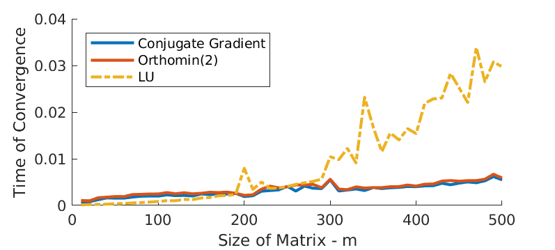
Figure 8 - Log-scale residual over iterations.
Note that above analysis is based on the \(1000 \times 1000\) matrix \(A\) whose eigenvalues form a linear span from 1 to 2. The eigenvalues of \(A\) has very narrow range and are distributed uniformly. To see how the convergence can be impacted by the distributions of \(A\)’s eigenvalues, we regenerate \(A\) with differently distributed eigenvalues. In particular, we generate 4 \(A\) with eigenvalues that
- have uniform narrow range;
- have uniform wide range;
- have very large and small value;
- have repeated value.
Next we apply the Conjugate Gradient algorithm to solve \(Ax=b\), and obtain the convergence rate shown in Figure 9. First of all, if \(A\)’s eigenvalues contain very large eigenvalues (e.g. the largest one is \(10^8\) times of the smallest), then the algorithm does not seem to converge at all (note in this example we allow at most \(10^6\) iterations). Narrow-ranged eigenvalues result in faster convergence than wide-ranged eigenvalues do. Repeated eigenvalues also tend to slow down the convergence.
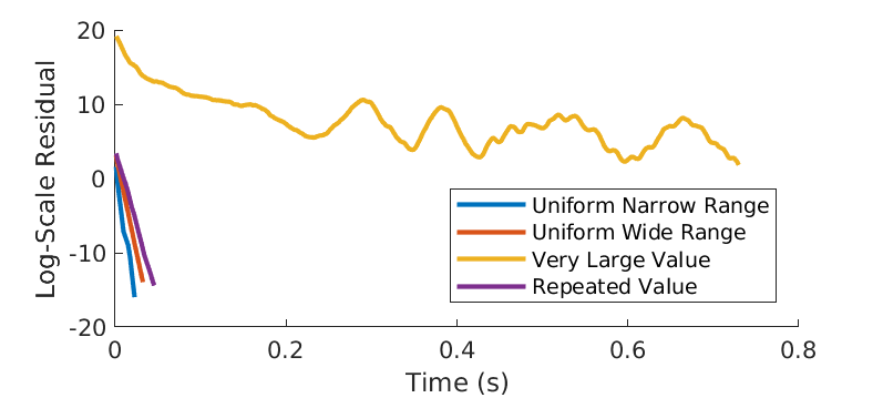
Figure 9 - Impact of distributions of eigenvalues.
Convergence performance of GMRES
The last iterative method we implement is the GMRES algorithm. In general, we consider GMRES as the last resort for solving linear system, since it does not require extra conditions on \(A\) but can be quite complex.
First, we analyse how the distribution of \(A\)’s eigenvalues influences the convergence of the algorithm. Consider a \(100\times 100\) symmetric matrix \(A\) where its eigenvalues are uniformly distributed within the range \([-c,c]\).
In Figure 10, we show the log-scale residual over iterations for the same GMRES algorithm given different \(A\), that is characterized by \(c\). Larger \(c\) implies that \(A\) has larger eigenvalues as well as a wider range of eigenvalues. Respectively, the convergence is expected to be slower for \(A\) with larger \(c\). This is confirmed by Figure 10.
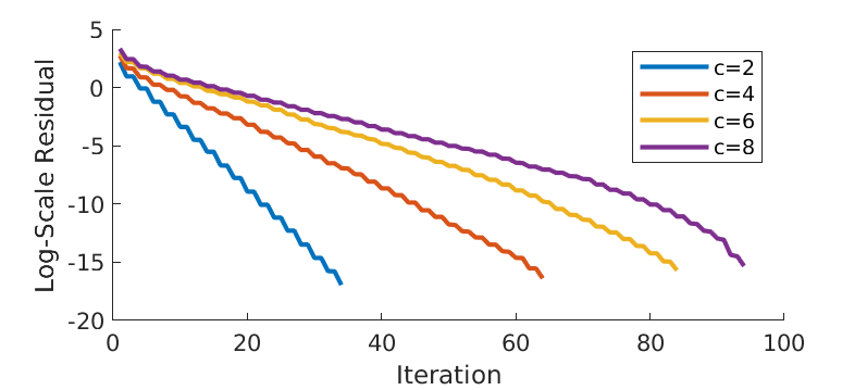
Figure 10 - Impact of distributions of eigenvalues.
We also compare the convergence performance of the GMRES with other algorithms for solving the same linear system. In particular, Figure 11 displays the time of convergence with \(m\), the size of the matrix. Still, the required time of convergence increases with matrix size. All the other 3 algorithms seem to outperform GMRES when \(m<200\). For matrix size \(m>200\), the MATLAB built in LU factorization is beaten by the others, and its associated time of convergence seem to grow at least quadratically. However, all the other algorithms only require linearly growing time for convergence as matrix size scale up. Overall, the GMRES algorithm always converges slower than the Orthomin(2) and Conjugate Gradient does.
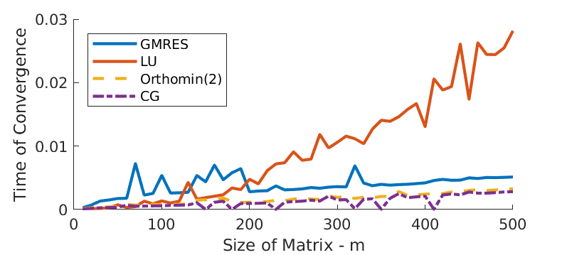
Figure 11 - Time of convergence.
SVD
In the section, we discuss SVD, the singular value decomposition, of the \(m\times n\) matrix \(A\).
We have implemented a two-step algorithms to decompose the matrix \(A\),
- Apply the Golub-Kahan bi-diagonalization to \(A\) and obtain an upper bi-diagonal matrix \(B\), as well unitary matrix \(U\) and \(V\).
- Apply the Cholesky iteration (dqds) to B and get the singular values.
Figure 12 shows a comparison between the results from our implementation dqds() and the MATLAB in-built svd() function. The singular values are ordered from the largest to the smallest from left to right. Visually the difference is small.
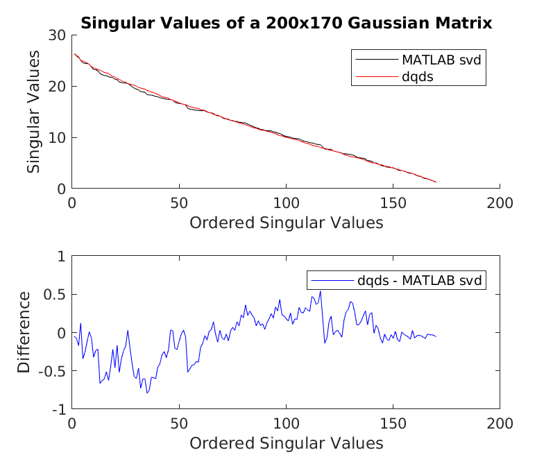
Figure 12 - Singular values comparison.
See below the MATLAB script of the dqds() function: