Sparse representation of signals with the K-SVD algorithm
We provide an executive summary of the paper by Michal Aharon, Michael Elad and Alfred Bruckstein
Sparse representations of signals
Suppose a signal is denoted by a numeric vector \(\mathbf{y} \in \mathbb{R}^n\), the sparse representation of the signal is \(\mathbf{y} \approx \mathbf{D} \mathbf{x}\), where \(\mathbf{D} \in \mathbb{R}^{n \times K}\) is called the overcomplete dictionary matrix assuming \(n < K\) and \(\mathbf{x} \in \mathbb{R}^K\) is a sparse vector. In other words, the goal is to represent \(\mathbf{y}\) as a sparse linear combination of the \(K\) prototype signal atoms \(\{\mathbf{d}_j\}^K_{j=1}\) that form columns of the dictionary \(\mathbf{D}\).
The application of sparse representation is to train a proper dictionary \(\mathbf{D}\) based on a set of signals \(\mathbf{Y} = \{\mathbf{y}_j\}_{j=1}^N\), so that all newly coming signals can be possibly stored at minimum space as a sparse vector by taking advantage of this dictionary. This can be formulated as,
\[\begin{equation} \min_{\mathbf{D}, \mathbf{X}} \left\{ ||\mathbf{Y} - \mathbf{DX}||_F^2 \right\}, \text{ s.t. } \forall i, ||\mathbf{x}_i||_0 \leq T_0, \label{eq:formula} \end{equation}\]where \(\mathbf{X} = \{\mathbf{x}_i\}_{i=1}^{N} \in \mathbb{R}^{K \times N}\), and \(T_0\) defines the sparsity requirement. The objective targets to minimise the Frobenius norm by optimising the choice of dictionary \(\mathbf{D}\) and sparse matrix \(\mathbf{X}\).
The algorithms of solving the sparse representation problem (\ref{eq:formula}) typically involves iteratively solving \(\mathbf{X}\) and \(\mathbf{D}\) in sequence, given the other variable as a known parameter. In fact, literatures denote the corresponding two subproblems,
-
Sparse coding is to compute the representation coefficients \(\mathbf{x}\) based on the given signal \(\mathbf{y}\) and the dictionary \(\mathbf{D}\) by solving \eqref{eq:formula}.
-
Dictionary update is to search for better dictionary \(\mathbf{D}\) based on the given signals \(\mathbf{Y}\) and the solved coefficients matrix \(\mathbf{X}\) in the previous sparse coding stage. By “better” we mean to further minimise the objective in \eqref{eq:formula}.
The K-SVD algorithm
The K-SVD algorithm introduced by Michal Aharon, Michael Elad and Alfred Bruckstein
To see this, we assume that both \(\mathbf{X}\) and \(\mathbf{D}\) are fixed, and we would like to update only one column of dictionary \(\mathbf{d}_k\), and the associated sparse representations \(\mathbf{x}^k_T\), namely the \(k\)-th row in \(\mathbf{X}\). Then the objective in (\ref{eq:formula}) is rewritten as,
\[\begin{align} ||\mathbf{Y} - \mathbf{D} \mathbf{X}||_F^2 & = \left\Vert \left( \mathbf{Y} - \sum_{j \neq k} \mathbf{d}_j \mathbf{x}^k_T \right) - \mathbf{d}_k \mathbf{x}_T^k \right\Vert_F^2 \\ & := \left\Vert \mathbf{E}_k - \mathbf{d}_k \mathbf{x}_T^k \right\Vert_F^2. \label{eq:errorUpdateD} \end{align}\]The matrix \(\mathbf{E}_k\) represents the error for all the \(N\) samples when the \(k\)-th atom is removed. We can use SVD to find the closest rank-1 matrix that approximates \(\mathbf{E}_k\), which effectively minimizes (\ref{eq:errorUpdateD}). However, the resulting \(\mathbf{x}_T^k\) is unlikely to fulfil the sparsity requirements. The remedy is to require that the new \(\tilde{\mathbf{x}}_T^k\) to have the same support as the original \(\mathbf{x}_T^k\). To add the requirement, we revise the objective (\ref{eq:errorUpdateD}) to
\begin{equation} \left\Vert \mathbf{E}_k \mathbf{\Omega}_k - \mathbf{d}_k \mathbf{x}_T^k \mathbf{\Omega}_k \right\Vert_F^2, \end{equation} where
\[\begin{equation} \mathbf{\Omega}_k = \begin{cases} 1 \text{, } i = \omega_k(j); \\ 0 \text{, otherwise;} \end{cases} \end{equation}\]and that the support of \(\mathbf{x}_T^k\) is defined as \(\omega_k := \{i: 1 \leq i \leq K, \text{ } \mathbf{x}_T^k \neq 0 \}\). Multiplying \(\mathbf{\Omega}_k\) shrinks \(\mathbf{x}_T^k\) by discarding zero entries and also refines \(\mathbf{E}_k\) to a selection of error columns that correspond to samples that use the atom \(\mathbf{d}_k\).
Thereafter, we can decompose \(\mathbf{E}_k \mathbf{\Omega}_k = \mathbf{U} \Delta \mathbf{V}^\top\), and update:
-
\(\mathbf{d}_k\) as the first column of \(\mathbf{U}\);
-
the non-zero elements of \(\mathbf{x}_T^k\) as the first column of \(\mathbf{V}\) multiplied by the largest singular value, namely \(\Delta (1,1)\)
By far, the K-SVD algorithm completes updating the dictionary, which will be used in the next iteration for sparse coding, unless the convergence requirement is satisfied (or maximum iterations is reached).
Synthetic experiments
We’ve implemented the K-SVD algorithm in Python (see the Appendix). Meanwhile, we solve the sparse coding problem by taking advantage of the OrthogonalMatchingPursuit() implementation maintained by Scikit-learn. Together we are able to iteratively solve the sparse representation problem.
To test the algorithm and our implementation, we follow the same way as described in \cite{aharon} to simulate synthetic data (section V.A.) and measure performance (equation (25) in section V.D.). Moreover, we define a more general performance measure
\[\begin{equation} P(\epsilon) = \sum_{k=1}^K \mathbf{1}_{\{1-|\mathbf{d}_i^\top \tilde{\mathbf{d}}_i|< \epsilon \} }, \label{eq:performance} \end{equation}\]which counts the number of “successes” in recovering the dictionary. Here \(\mathbf{d}_i\) is the generating dictionary atom and \(\tilde{\mathbf{d}}_i\) is its corresponding element (closest column in \(\ell^2\) norm) in the recovered dictionary.
We need to initialise a dictionary to feed into the sparse coding process. Therefore it is reasonable to investigate the sensitivity of the result against the dictionary initialisation. Nevertheless, we show the result from one single trial first. In Figure 1, we plot the relative error (\(\|\mathbf{Y}-\mathbf{DX}\|_F / \|\mathbf{Y}\|_F\)) over iterations on the left, and the histogram of column \(\ell^2\)-norm errors on the right. The errors tend to converge into a positive constant. More than that, dictionary update by K-SVD algorithm greatly reduces the error during each iteration. Unfortunately, the orthogonal matching pursuit algorithm in the next iteration always brings the error back to a high level. We are thinking that this could be caused by that the function implemented by Skicit-learn does not allow us to initialize \(\mathbf{X}\) from previous iteration, so that it always leads to another worse local minimum. Looking at the histogram, we observe that 95% of the recovered signals (columns) have less than 20% errors from the original signals.
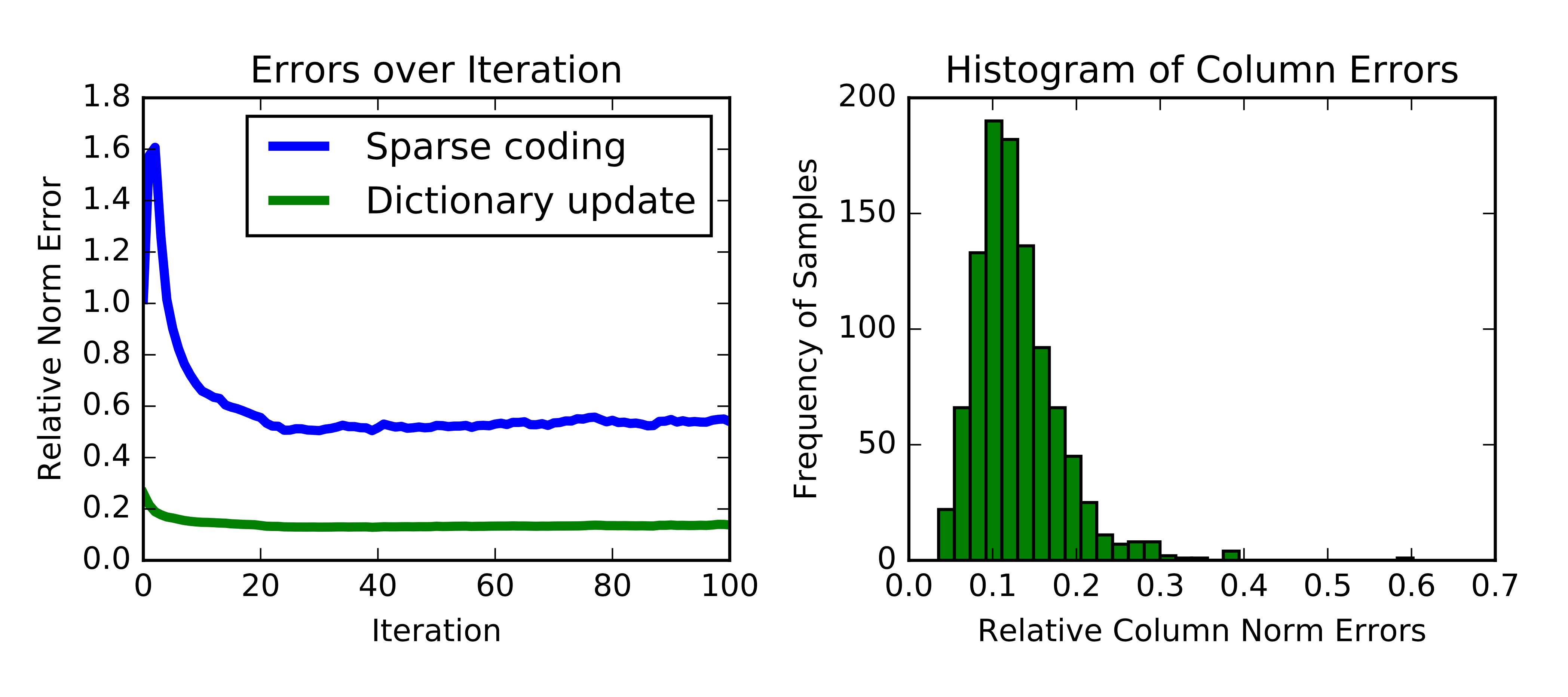
Figure 1 - Error.
Next we look at the performance measure as defined in (\ref{eq:performance}). In Figure 2, we show how the number of successes vary with tolerance. With \(\epsilon \geq 0.06\), we can obtain at least 45 successes out of 50 for dictionary recovery.
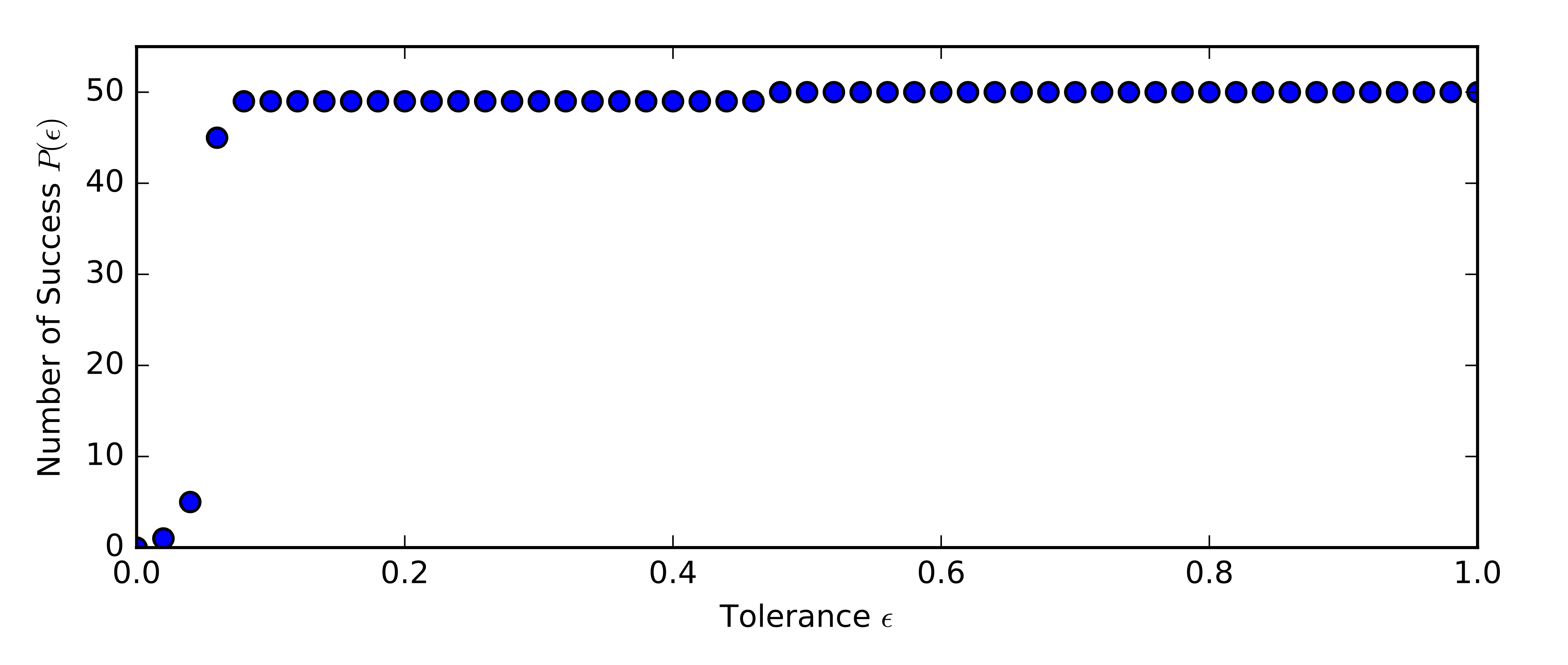
Figure 2 - Count of successes.
As mentioned before, it is reasonable to investigate the sensitivity of the result against the dictionary initialization. We initialize the dictionary with i.i.d. uniformly distributed entries. Each column is then normalized to a unit \(\ell^2\)-norm. We show in Figure 3 how error evolves over iterations for 50 different initialisation. It turns out the errors are reasonably consistent by the end of iteration.
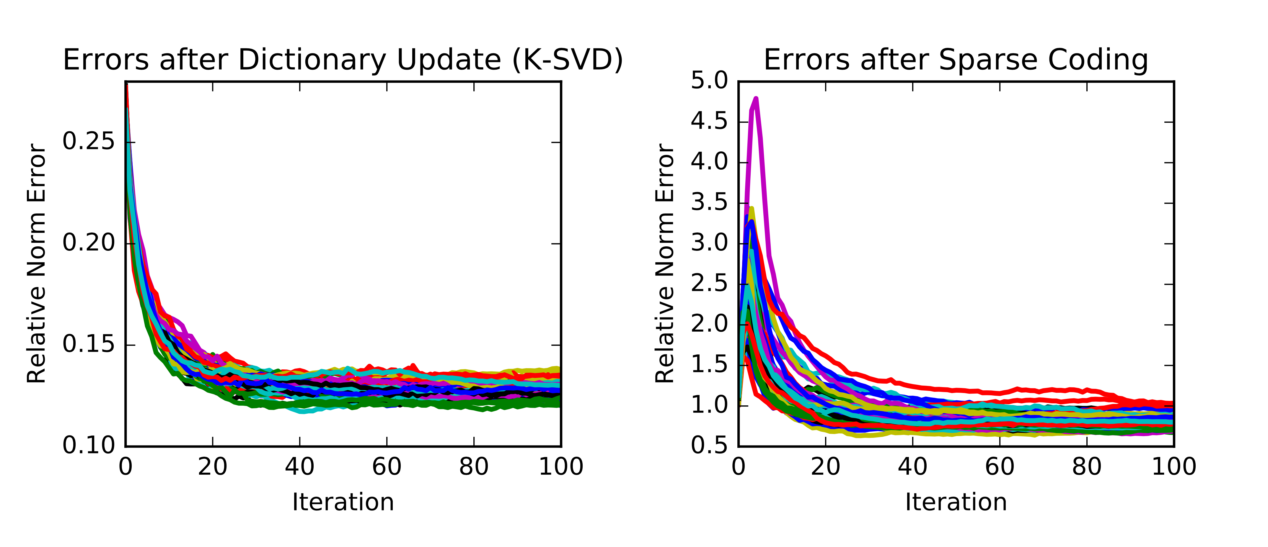
Figure 3 - Errors of multiple trials.
Appendix
import numpy as np
import scipy as sp
import scipy.sparse as sps

from scipy.linalg import norm, svd
from scipy.stats import rankdata

from sklearn.linear_model import OrthogonalMatchingPursuit

import matplotlib.pyplot as plt

def gen_rand_dict_mat(n_features, n_atoms):
  '''
  Simulate dictionary D with unit-L2-norm column.

  Arguments:

      n_features: int
          Number of features for signals

      n_atoms: int
          Number of signal atoms in the dictionary D.

  Returns:

      D: 2-D matrix, shape=(n_features, n_atoms)
          Simulated dictionary
  '''

  D_raw = np.random.rand(n_features, n_atoms)
  col_norms = norm(D_raw, ord=2, axis=0)
  D = D_raw / col_norms

  return np.mat(D)

def gen_rand_measure(n_samples, n_atoms, n_sparsity):
  '''
  Simulate sparse representation coefficient matrices X. The number of non-zero
  elements equals to n_sparsity, their values are uniformly distributed in
  interval [0.1], and their locations are also uniformly random.

  Arguments:

      n_samples: int
          Number of samples

      n_atoms: int
          Number of signal atoms in the dictionary D.

      n_sparsity: int
          Maximal number of non-zero elements allowed in each measurment vector.

  Returns:

      X: 2-D sparse matrix, shape=(n_atoms, n_samples)
          Each column contains the coefficients for sparse representation of signals.
  '''
  X = np.zeros([n_atoms, n_samples])

  for m in range(n_samples):
      temp = np.random.rand(n_atoms)
      rank = rankdata(temp) - 1
      loc_indices = rank[0 : n_sparsity]

      vals = np.random.rand(n_sparsity)

      for (idx, val) in zip(loc_indices, vals):
          X[int(idx),m] = val

  # Compressed Sensing Column (CSC) matrix
  return sps.csc_matrix(X)

def calc_errors_pctile(Y, Y_backup, pct):
  error_list = norm(Y - Y_backup, ord=2, axis=0)
  return np.percentile(error_list, pct)

def accuracy(D, D_generating, tol=0.1):
  _, k_codewords = D.shape

  correct = 0

  for k in range(k_codewords):
      for j in range(k_codewords):
          if 1 - np.abs((D[:,j]).transpose()*D_generating[:,k]) < tol:
              correct += 1
              break

  return correct

def calc_ksvd(Y, n_atoms, n_sparsity, max_iter=100, tol=1e-2, pct = 95):
  '''
  Arguments:

      Y: 2-D matrix, shape = (n_features, n_samples)
          Original signals, each column represents a signal.

      n_atoms: int
          Number of signal atoms in the dictionary D.

      n_sparsity: int
          Maximal number of non-zero elements allowed in each measurment vector.

      max_iter: int
          Maximal number of iterations allowed.

      tol: float
          Tolerance of convergence measured as L-2 norm ||y-Dx||_2 for one signal.

      pct: float
          Percentile of norm errors over signals. Convergence is reached if the
          pct-th percentile of signal norm error is less than tol.

  Returns:

      D: 2-D matrix, shape = (n_features, n_atoms)
          Dictionary of signal atoms.

      X: 2-D sparse matrix, shape = (n_atoms, n_samples)
          Each column contains the coefficients for sparse representation of
          signals.

      err_sparse_coding: dictionary(key:int, value:float)
          Dictionary with keys being iteration count, values being norm error
          after sparse coding.

      err_dict_update: dictionary(key:int, value:float)
          Dictionary with keys being iteration count, values being norm error
          after dictionary update.
  '''

  n_features, n_samples = Y.shape

  # Initialize dictionary
  D_0 = gen_rand_dict_mat(n_features, n_atoms)
  iter_count = 0
  err_sparse_coding = {}
  err_dict_update = {}

  D = D_0
  while True:
      iter_count = iter_count + 1
      if iter_count > max_iter:
          break

      # Sparse coding
      omp = OrthogonalMatchingPursuit(n_nonzero_coefs=n_sparsity)
      omp.fit(D, Y)
      X = sps.csc_matrix(omp.coef_.transpose())
      err_sparse_coding[iter_count] = norm(Y-D*X)
      print("Iteration = {}/{}, Sparse Codeing - Columm-Pct Norm error = {}".
            format(iter_count, max_iter, calc_errors_pctile(Y, D*X, pct)))

      # Codebook update
      for k in range(n_atoms):
          xk = X[k,:]
          DX_k = D*X - D[:,k]*xk
          E = Y - DX_k

          nonzero_idx = np.nonzero(xk)
          nonzero_size = len(nonzero_idx[1])
          ones = np.ones(nonzero_size)
          Omega = sps.csc_matrix((ones, (nonzero_idx[1], range(nonzero_size))),
                                 shape=(n_samples, nonzero_size))

          E_Omega = E * Omega
          xk_Omega = xk * Omega

          U, s, Vh = svd(E_Omega, full_matrices=False)
          dk = U[:,0]
          xk_Omega = s[0]*Vh[0,:]
          xk = sps.csc_matrix((xk_Omega, (np.zeros(nonzero_size),
                               nonzero_idx[1])), shape=(1, n_samples))

          # Update X_J
          X[k,:] = xk
          # Update D_J
          D[:,k] = np.mat(dk).T

      err_dict_update[iter_count] = norm(Y-D*X)
      err = calc_errors_pctile(Y, D*X, pct)
      print('Iteration = {}/{}, Dict Update    - Columm-Pct Norm error = {}'.
            format(iter_count, max_iter, err))

      # Termination condition
      if err < tol:
          break

  return D, X, err_sparse_coding, err_dict_update

def main():

  # Simulate test data
  # Y.shape = (n, N)
  # D.shape = (n, K)
  # X.shape = (K, N)
  np.random.seed(100)
  n, K, N, n_sparsity = 20, 50, 1000, 3
  D = gen_rand_dict_mat(n, K)
  X = gen_rand_measure(N, K, n_sparsity)
  Y = D * X

  # Run K-SVD and store results
  n_sim = 1
  max_iter = 20
  tol = 1e-2
  pct = 95
  result_D = []
  result_X = []
  result_errsc = []  # error after sparse coding
  result_errdu = []  # error after dictionary update
  for i_sim in range(n_sim):
      D_J, X_J, err_sparse_coding, err_dict_update = calc_ksvd(
        Y, K, n_sparsity, max_iter=max_iter, tol=tol, pct=pct)
      result_D.append(D_J)
      result_X.append(X_J)
      result_errsc.append(err_sparse_coding)
      result_errdu.append(err_dict_update)

  # Display results for a particular simulation
  idx = 0  # the first simulation
  D_J = result_D[idx]
  X_J = result_X[idx]
  err_sparse_coding = result_errsc[idx]
  err_dict_update = result_errdu[idx]

  d_accuracy_tol = 0.07
  success = accuracy(D, D_J, d_accuracy_tol)
  print('With tolerance = {}. The number of success = {} out of {}'.\
    format(d_accuracy_tol, success, K))

  plt.figure()
  error_list = norm(Y - D_J * X_J, ord=2, axis=0)
  norm_list = norm(Y, ord=2, axis=0)
  rel_err_list = error_list / norm_list
  plt.hist(rel_err_list, bins=25, alpha=0.5)
  plt.xlabel('Relative Column Norm Errors')
  plt.ylabel('Frequency of Samples')
  plt.title('Histogram of Column Errors')

  plt.figure()
  plt.plot(err_sparse_coding.values() / norm(Y), label='Sparse coding', linewidth=2)
  plt.plot(err_dict_update.values() / norm(Y), label='Dictionary update', linewidth=2)
  plt.xlabel('Iteration')
  plt.ylabel('Relative Norm Error')
  plt.title('Errors over Iteration')
  plt.legend()

  plt.show()

if __name__ == "__main__":
  main()