Mixed finite element method - solving a linear elasticity coupled with diffusion problem
We apply the mixed finite element method (see, for example, Gatica
Since it requires intensive notations for function spaces to define weak formulations and discuss sovability, we summarize the notations of key function spaces in Appendix for reference.
Linear elasticity with diffusive body force
Let \(\Omega\) be a bounded domain of \(\mathbb{R}^n\), \(n \geq 2\), with Lipschitz-continuous boundary \(\Gamma\). The linear elasticity problem targets to solve the displacement \(\mathbf{u}\) and the stress tensor \(\sigma\) of an elastic material occupying the region \(\Omega\), such that,
\[\sigma = \mathcal{C} \varepsilon (\mathbf{u}) \quad \text{in } \Omega,\]\begin{equation} -\nabla \cdot \sigma = \mathbf{f} \quad \text{in } \Omega, \label{eq:linearElasticity} \end{equation}
where \(\mathbf{f} \in [L^2(\Omega)]^n\) is the body force per unit volume, \(\varepsilon (\mathbf{u}) : = \frac{1}{2} \left[ \nabla \mathbf{u} + (\nabla \mathbf{u})^\top \right]\) is the strain tensor, and \(\mathcal{C}\) is the elasticity operator given by Hooke’s law, that is, \begin{equation} \mathcal{C} \zeta = \lambda \text{tr} (\zeta) \mathbf{I} + 2 \mu \zeta \quad \forall \zeta \in [L^2 (\Omega)]^{n \times n}. \end{equation} Here, \(\lambda, \mu>0\) are the respective Lam'e constants, \(\mathbf{I}\) is the identity matrix of \(\mathbb{R}^n\), and tr(\(\cdot\)) is the matrix trace.
We introduce diffusion term into the body force term by letting \(\mathbf{f} = \mathbf{f} (\phi)\), with \(\phi\) being the solution of a diffusion problem
\begin{equation} -\nabla \cdot (D(\sigma) \nabla \phi) = g. \label{eq:diffusion} \end{equation}
Here we assume \(g \in L^2(\Omega)\) and that the diffusivity \(D\) depends on the stress tensor \(\sigma\). As a result, the linear elasticity problem (\ref{eq:linearElasticity}) and the diffusion problem (\ref{eq:diffusion}) have to be solved simultaneously.
We consider a simple set-up for the boundary conditions of both problems, where there are only Dirichlet boundaries. In particular, we let
\begin{equation} \mathbf{u} = \mathbf{0} \quad \text{on } \Gamma, \label{eq:bcLE} \end{equation}
\begin{equation} \phi = \phi_D \quad \text{on } \Gamma. \label{eq:bcD} \end{equation}
Weak formulation and solvability
We derive the weak formulation for the linear elasticity problem (\ref{eq:linearElasticity}) and the diffusion problem (\ref{eq:diffusion}) by incorporating the Dirichlet boundary conditions (\ref{eq:bcLE}) and (\ref{eq:bcD}), and then state the solvability of the system of problems.
\paragraph{Weak formulation of the linear elasticity problem}
We introduce an auxiliary unknown \(\rho\) named rotation of the material by \begin{equation} \rho := \frac{1}{2} \left[ \nabla \mathbf{u} - (\nabla \mathbf{u})^\top \right], \end{equation}
which by construction implies that \(\rho \in L^2\_\text{skew} (\Omega)\), where
\begin{equation} L^2_\text{skew}(\Omega) := \Big\{ \eta \in [L^2(\Omega)]^{n\times n} : \eta + \eta^\top = 0 \Big\}. \end{equation}
Thereafter, we obtain the following weak formulation:
Find \((\sigma, (\mathbf{u}, \rho)) \in H \times Q\) such that \begin{equation} a(\sigma, \tau) + b(\tau, (\mathbf{u}, \rho)) = F(\tau) \forall \tau \in H \label{eq:weakLE0} \end{equation} \begin{equation} b(\sigma, (\mathbf{v}, \eta)) = G(\mathbf{v}, \eta) \forall (\mathbf{v}, \eta) \in Q, \end{equation} where the two function spaces \(H\) and \(Q\) are defined by \begin{equation} H := \{ \tau \in [L^2(\Omega)]^{n \times n} : \nabla \cdot \tau \in [L^2(\Omega)]^n, \int_\Omega \text{tr}(\tau) = 0 \}, \end{equation} \begin{equation} Q := [L^2(\Omega)]^n \times L^2_\text{skew}(\Omega), \end{equation} and the bilinear forms \(a:H\times H \mapsto \mathbb{R}\) and \(b:H\times Q \mapsto \mathbb{R}\) are defined by \begin{equation} a(\zeta, \tau) := \frac{1}{2\mu} \int_\Omega \Big( \zeta:\tau - \frac{\lambda}{n\lambda + 2\mu} \text{tr}(\zeta) \text{tr}(\tau) \Big), \end{equation} \begin{equation} b(\sigma, (\mathbf{v}, \eta)) := \int_\Omega \mathbf{v} \cdot \nabla \cdot \tau + \int_\Omega \eta : \tau, \end{equation} and the functionals \(F\) and \(G\) are given by \begin{align} F(\tau) := 0, \quad G(\mathbf{v}, \eta) := - \int_\Omega \mathbf{f} \cdot \mathbf{v}. \label{eq:weakLE} \end{align}
Weak formulation of the diffusion problem
Since the boundary condition (\ref{eq:bcD}) is inhomogeneous, we set \(\phi = \hat{\phi} + \phi_D\) and solve \(\hat{\phi}\) instead. By letting \(\phi_D\) be a constant, we obtain the following weak formulation:
Find \(\hat{\phi} \in V\) such that \begin{align} c(\hat{\phi},v) & = L(v) & \forall v \in V, \label{eq:weakD0} \end{align} where the function space \(V\) is defined by \begin{align} V & := \Big\{ v \in H^1(\Omega) : v = 0 \text{ on } \Gamma \Big\}, \label{eq:defV} \end{align} and the bilinear forms \(L:V\times V \mapsto \mathbb{R}\) is defined by \begin{align} c(u, v) & := \int_\Omega D(\sigma) \nabla \hat{\phi} \cdot \nabla v , \end{align} and the functional \(L\) is given by \begin{align} L(v) & := \int_\Omega g v \label{eq:weakD} \end{align}
Solving strategy for the system of problems
Because the weak formulations of linear elasticity problem (\ref{eq:weakLE0})-(\ref{eq:weakLE}) and the diffusion problem (\ref{eq:weakD0})-(\ref{eq:weakD}) interact with each other, all the unknowns have to be solved simultaneously. To solve them, we define a fixed-point problem:
We fix a solution of the diffusion problem (\ref{eq:weakD}), \(\hat{\phi}\), and define the solution operator for the linear elasticity problem (\ref{eq:weakLE}) as \begin{align} \mathcal{S}_E (\hat{\phi}) = (\sigma, (\mathbf{u}, \rho)) \quad \forall \hat{\phi} \in V. \label{eq:fixpoint0} \end{align} Similarly, we fix a solution of the linear elasticity problem, \((\sigma, (\mathbf{u}, \rho))\), and define the solution operator for the diffusion problem as \begin{align} \mathcal{S}_D (\sigma, (\mathbf{u}, \rho)) = \hat{\phi} \quad \forall (\sigma, (\mathbf{u}, \rho)) \in H \times Q. \end{align} Finally, define \(T: V \mapsto V\) by \begin{align} T(\hat{\phi}) = \mathcal{S}_D (\mathcal{S}_E (\hat{\phi})) \quad \forall \hat{\phi} \in V, \end{align} such that our goal is to solve the following fixed-point equation \begin{align} T(\hat{\phi}) = \hat{\phi}. \label{eq:fixpoint} \end{align}
Discussion on the solvability
The solvability of the problem (\ref{eq:fixpoint0})-(\ref{eq:fixpoint}) depends on the solvability of three subproblems, namely the linear elasticity problem (\ref{eq:weakLE}) given \(\hat{\phi}\), the diffusion problem (\ref{eq:weakD}) given \((\sigma, (\mathbf{u}, \rho))\), and eventually the fixed-point equation (\ref{eq:fixpoint}).
We start from the easier diffusion problem. The Lax-Milgram theorem guarantees the existence and uniqueness of the solution of (\ref{eq:weakD}) because we can show that
-
\(V\) defined in (\ref{eq:defV}) is a closed subspace of \(H^1(\Omega)\), and \(H^1(\Omega)\) with the norm \(\|v\|^2_{1,\Omega} := \|v\|^2_{L^2(\Omega)} + \|\nabla v\|^2_{L^2(\Omega)}\) is a Hilbert space;
-
\(c(\cdot, \cdot)\) is coercive on \(H^1(\Omega) \times H^1(\Omega)\) (Cauchy-Schwarz inequality);
-
\(c(\cdot, \cdot)\) is bounded on \(H^1(\Omega) \times H^1(\Omega)\) (Poincar'e inequality);
-
\(L(\cdot)\) is bounded on \(H^1(\Omega)\) (Cauchy-Schwarz inequality).
The linear elasticity problem involves mixed formulations, where Lax-Milgram theorem needs to be adapted to apply for demonstrating the solvability. In summary, we can prove the well-posedness of (\ref{eq:weakLE}) by showing that
-
\(H\) and \(Q\) are Hilbert spaces;
-
\(a(\cdot, \cdot)\) is bounded on \(H \times H\), \(b(\cdot, \cdot)\) is bounded on \(H \times Q\);
-
\(F(\cdot)\) is bounded on \(H\), \(G(\cdot)\) is bounded on \(Q\);
-
\(a(\cdot, \cdot)\) is coercive on \(K\) which is defined by
\begin{equation} K := { \tau \in H : b(\sigma, (\mathbf{v}, \eta)) = 0 \quad \forall (\mathbf{v}, \eta) \in Q }; \label{eq:kerlB} \end{equation} \item \(b(\cdot, \cdot)\) satisfies the inf-sup condition, that is, \(\exists c_b >0\) such that \begin{equation} c_b \leq \inf_{(\mathbf{v}, \eta) \in Q \backslash { (\mathbf{0}, \mathbf{0}) }} \sup_{\tau \in H \backslash {\mathbf{0}}} \frac{b(\tau, (\mathbf{v}, \eta))}{||\tau||_H ||(\mathbf{v}, \eta)||_Q} ; \end{equation}
The last piece is to show the fixed-point equation (\ref{eq:fixpoint}) yields a root. In fact, fixed-point theorem confirms the existence of a solution if we show that \(T(\cdot)\) is continuous from a solution space \(W\) into itself, and that \(T(W)\) is a relatively compact subspace of \(W\). To define \(W\), we recall that the well-posedness of the diffusion problem also indicates that \(\|\hat\phi\|_{1,\Omega} \leq C \|L\|_{H^1(\Omega)'} \leq C_{\phi}\) for some constant \(C_\phi\). Thereafter, we can define the solution space for \(\hat{\phi}\) as
\begin{equation} W = \Big\{ v \in H^1(\Omega) : ||v||_{1,\Omega} \leq C_\phi \Big\}. \end{equation}
Hence, we show that
-
\(T(W) \subset W\);
-
The continuity of \(T\), that is, \(\forall \phi, \varphi \in W\)
\begin{equation} ||T(\phi) - T(\varphi)||_{1,\Omega} \leq C ||\phi - \varphi||_{1,\Omega}. \end{equation}
Discrete formulation - Galerkin Approximation and Fixed-Point Iteration
Suppose \(H_h \subset H\), \(Q_h \subset Q\) and \(V_h \subset V\) are linear subspaces of the corresponding Hilbert spaces. The discrete Galerkin approximation of the linear elasticity problem weak formulation (\ref{eq:weakLE0})-(\ref{eq:weakLE}) is:
Find \((\sigma_h, (\mathbf{u}_h, \rho_h)) \in H_h \times Q_h\) such that \begin{align} a(\sigma_h, \tau_h) + b(\tau_h, (\mathbf{u}_h, \rho_h)) = F(\tau_h) \text{ }\forall \tau_h \in H_h \label{eq:galerkinLE0} \end{align} \begin{align} b(\sigma_h, (\mathbf{v}_h, \eta_h)) = G(\mathbf{v}_h, \eta_h) \quad \forall (\mathbf{v}_h, \eta_h) \in Q_h. \label{eq:galerkinLE} \end{align}
And the Galerkin approximation of the diffusion problem weak formulation (\ref{eq:weakD0})-(\ref{eq:weakD}) is:
Find \(\hat{\phi}_h \in V_h\) such that \begin{align} c(\hat{\phi}_h,v_h) & = L(v_h) & \forall v_h \in V_h. \label{eq:galerkinD} \end{align}
Finally, we solve the fixed-point equation using the following iterative method:
Algorithm Fixed-Point Iteration:
initialize \(\phi_h^0\), \(k=0\)
iterate until
res\(<\)tolupdate \(k = k+1\);
solve (\ref{eq:galerkinLE0})-(\ref{eq:galerkinLE}) using \(\phi_h^{k-1}\) \(\rightarrow\) \((\sigma_h^k, (\mathbf{u}_h^k, \rho_h^k))\) ;
solve (\ref{eq:galerkinD}) using \(\sigma_h^{k-1}\) \(\rightarrow\) \(\phi_h^k\) ;
define
res= \(\| \phi_h^{k-1} - \phi_h^{k}\|_{L^\infty} + \| \sigma^{k-1} - \sigma^{k}\|_{L^\infty}\);return \(\phi_h^k\), \((\sigma_h^k, (\mathbf{u}_h^k, \rho_h^k))\)
Discussion on the solvability
The fixed-point theorem guarantees that the iteration algorithm can find a root. It remains to show the solvability of the Galerkin approximation for two problems (\ref{eq:galerkinLE0})-(\ref{eq:galerkinLE}) and (\ref{eq:galerkinD}).
For the diffusion problem (\ref{eq:galerkinD}), because \(c(\cdot, \cdot)\) and \(F(\cdot)\) satisfy the conditions of the Lax-Milgram Theorem, it can be shown that the Galerkin approximation is well-posed for any closed subspace \(V_h \subset V\). Moreover, C'ea’s lemma further states that the approximation error \(\|\hat{\phi} - \hat{\phi}\_h\|_V\) is bounded in terms of the best approximation errors \(\inf_{v_h \in V_h} \|\hat{\phi} - v_h\|_V\).
The discrete mixed formulation (\ref{eq:galerkinLE0})-(\ref{eq:galerkinLE}) of the linear elasticity problem is not granted solvability despite all the conditions satisfied in the continuous problem. We additionally restrict the choice of Galerkin subspaces so that the following conditions shall be met
-
\(a(\cdot, \cdot)\) is coercive on \(K_h\) which is defined by \begin{equation} K_h := { \tau_h \in H_h : b(\sigma_h, (\mathbf{v}_h, \eta_h)) = 0 \text{ } \forall (\mathbf{v}_h, \eta_h) \in Q_h }; \label{eq:kerlBh} \end{equation}
-
\(b(\cdot, \cdot)\) satisfies the inf-sup condition adapted to the subspaces \((H_h, Q_h)\), that is, \(\exists c_b >0\) such that \begin{equation} c_b \leq \inf_{(\mathbf{v}_h, \eta_h) \in Q_h \backslash { (\mathbf{0}, \mathbf{0}) }} \sup_{\tau_h \in H_h \backslash {\mathbf{0}}} \frac{b(\tau_h, (\mathbf{v}_h, \eta_h))}{||\tau_h||_H ||(\mathbf{v}_h, \eta_h)||_Q}; \end{equation}
Thereafter, we can conclude that there is a unique solution pair \((\sigma_h, (\mathbf{u}\_h, \rho_h)) \in H_h \times Q_h\) to (\ref{eq:galerkinLE}). Moreover, the error \(\|\sigma - \sigma_h\|_H + \|(\mathbf{u}, \rho)-(\mathbf{u}\_h, \rho_h)\|_Q\) is bounded in terms of the best approximation error \(\inf_{\tau_h \in H_h} \|\sigma - \tau_h\|_H\) and \(\inf_{(\mathbf{v}_h, \tau_h) \in Q_h} \|(\mathbf{u}-\rho) - (\mathbf{v}_h, \tau_h)\|_Q\).
Numerics
We show an implementation of solving a two-dimension linear elasticity with diffusive body force problem using FEniCS package. In Table 1, we list all parameters and their values assigned in the implementation.
| Param | Description | Value |
|---|---|---|
| \(n\) | Dimension | \(2\) |
| \(\Omega\) | Domain | \((x,y) \in ([0, 40], [0, 40])\) |
| \((\lambda, \mu)\) | Lame constants | \((4, 1)\) |
| \(\mathbf{f}(\phi)\) | Body force | \((\sin 2\pi x, 0) \phi\) |
| \(D(\sigma)\) | Diffusivity | \(\mathbf{I} + 0.01*\sigma\) |
| \(g\) | Diffusion source | 0.01 |
| \(\phi_D\) | Diffusion boundary | 1 |
| FE for \(H_h\) | Finite element | BDM |
| FE for \(Q_h\) | Finite element | DG |
| FE for \(V_h\) | Finite element | CG |
tol | Residual tolerance | 5e-4 |
Table 1 - List of Parameters and Values
The solution for the displacement field \(\mathbf{u}\) is shown in Figure 1, where magnitudes of \(x\)-component and \(y\)-component are displayed separately.
In Figiure 2, we show the magnitudes of four components of the 2-dimensional stress tensor \(\sigma\). Note that \(\sigma\) is symmetric, verified by the same solution obtained for \(\sigma_{12}\) and \(\sigma_{21}\).
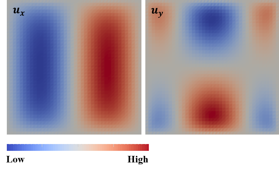
Figure 1 - Solution of \(\mathbf{u}\).
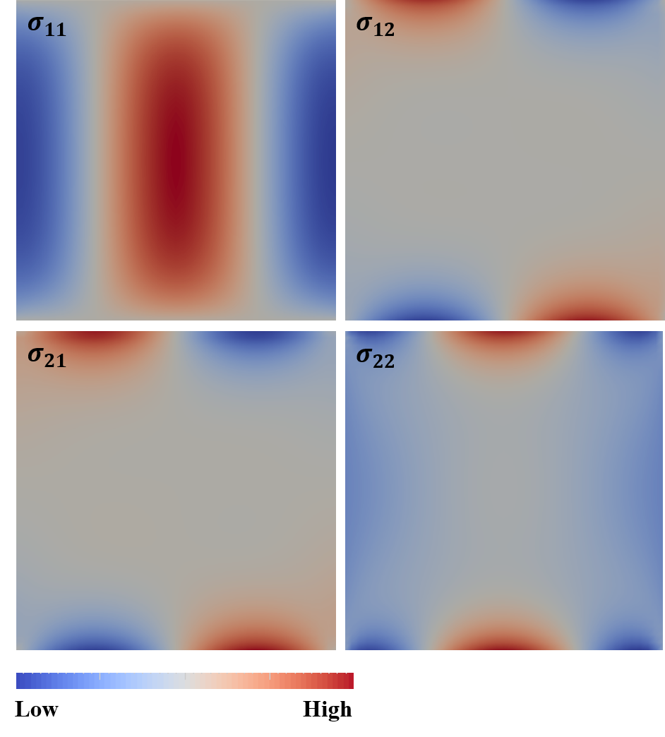
Figure 2 - Solution of \(\sigma\).
Appendix
Let \(\Omega\) be a bounded domain of \(\mathbb{R}^n\), \(n \geq 2\), with Lipschitz-continuous boundary \(\Gamma\). Here we summarise the definitions of relevant functions spaces \(\{u: \Omega \mapsto \mathbb{R} \}\) and their notations used throughout the paper.
Hilbert spaces
A Hilbert space \(H(\Omega)\) is a complete inner product space. Completeness means that all Cauchy sequences in \(H(\Omega)\) converge in \(H(\Omega)\).
Lebesgue spaces
For \(p \in [1, \infty]\), the \(L^p (\Omega)\) space is defined by
\[L^p(\Omega) = \left\{ u: \|u\|_{L^p(\Omega)} < \infty \right\},\]where the \(L^p\) norm is defined as
\[\|u\|_{L^p(\Omega)} = \left( \int_\Omega |u|^p \text{d}x \right)^{1/p} \quad p \in [1, \infty),\] \[\|u\|_{L^\infty(\Omega)} = \inf \left\{ C\geq 0: |u(x)| \leq C, \forall x \in \Omega \right\}.\]\(L^2\) space is also a Hilbert space, namely, \(L^2(\Omega) = H(\Omega)\).
Sobolev spaces
The Sobolev space \(W^k_p(\Omega)\), with non-negative integer \(k\) and \(p \in [1, \infty]\) is defined by
\[W^k_p(\Omega) = \left\{ u \in L_{loc}^1(\Omega) : \|u\|_{W^k_p(\Omega) < \infty} \right\},\]where \(L_{loc}^1(\Omega)\) denotes the set of locally integrable functions, and the Sobolev norm is defined as
\[\|u\|_{W^k_p(\Omega)} = \left( \sum_{|\alpha| \leq k} \|D^\alpha u\|_{L^p(\Omega)}^p \right)^{1/p} \quad p \in [1, \infty),\] \[\|u\|_{W^k_\infty(\Omega)} = \max_{|\alpha| \leq k} \|D^\alpha u\|_{L^\infty(\Omega)}.\]Here \(D^\alpha u\) denotes \(\alpha\)-th order of weak derivatives of \(u\).
Sobolev spaces
The Sobolev spaces with \(p=2\) are Hilbert spaces. These are denoted by
\[H^k(\Omega) = W_2^k (\Omega).\]Moreover, if we ask for no weak derivatives, the Sobolev space becomes \(L^p\) space, that is, \(W^0_p(\Omega) = L^p(\Omega)\). This in consequence leads to \(H^0(\Omega) = L^2(\Omega)\).